Back to Basic: Between Neural Network and Deep Neural Network

A neural network is a computational model inspired by the structure and functioning of the human brain. It consists of interconnected nodes, called neurons, organized into layers. Each neuron receives input signals, processes them, and produces an output signal. The strength of connections between neurons, represented by weights, determines how input signals are transformed into output signals.

A deep neural network (DNN) is a specific type of neural network characterized by having multiple hidden layers between the input and output layers. Deep neural networks are capable of learning complex patterns and representations from data, making them highly effective in tasks like image recognition, natural language processing, and more.

Here's a schematic diagram illustrating a simple neural network and a deep neural network:

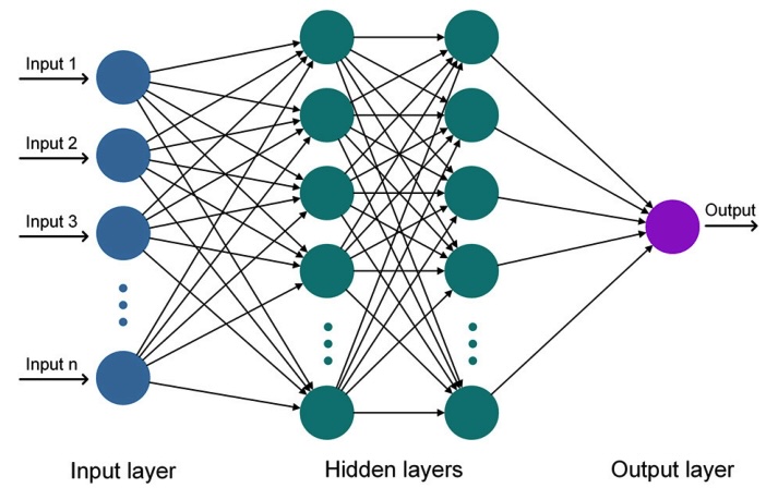
1. Schematic diagram of an Artificial Neural Network (ANN)

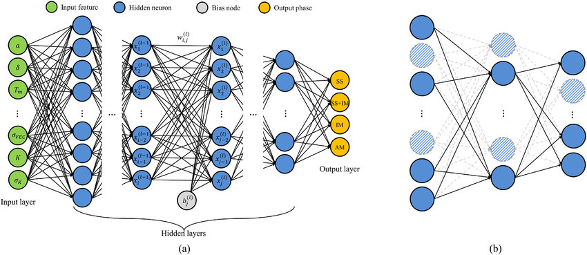
2. Schematic diagram of the deep neural network: (a) an architecture of DNN model comprised of input, hidden, and output layers (b) dropout regularization method that controls the connection of the neurons in the hidden layers.>

Neural Network

• Activation Function: Typically, the activation function used in neural networks is the sigmoid function or the rectified linear unit (ReLU) function.

The sigmoid function is given by:
$$[\sigma(x) = \frac{1}{1+e^{-x}} ]$$

The computation in a neural network with a sigmoid activation function involves the following steps:

1. Each neuron computes the weighted sum of its inputs:$$(z=\sum_{i=1}^{n} w_ix_i + b)$$ where$$(w_i)$$are the weights, $$(x_i)$$are the inputs, $$(b)$$is the bias, and$$(n)$$is the number of inputs.
2. The computed sum$$(z)$$is then passed through the activation function:$$(a=\sigma(z))$$ where$$(\sigma)$$is the sigmoid function.

Deep Neural Network

• Activation Function: Similar to neural networks, deep neural networks also use activation functions such as ReLU, sigmoid, or hyperbolic tangent (tanh).

The ReLU function is given by:
$$[f(x) = \max(0, x) ]$$

The computation in a deep neural network with ReLU activation function involves the following steps:

1. Each neuron computes the weighted sum of its inputs: $$( z = \sum_{i=1}^{n} w_ix_i + b )$$ where $$( w_i )$$ are the weights, $$( x_i )$$ are the inputs, $$( b )$$ is the bias, and $$( n )$$ is the number of inputs.
2. The computed sum $$( z )$$ is then passed through the ReLU activation function: $$( a = \max(0, z) )$$

These activation functions introduce non-linearity into the network, allowing it to learn complex relationships between inputs and outputs.

Each activation function serves different purposes and is suitable for different types of tasks within neural networks:

1. ReLU (Rectified Linear Unit):

   • Purpose: ReLU is widely used in deep neural networks because of its simplicity and effectiveness. It introduces non-linearity by outputting the input directly if it is positive, and zero otherwise.
   • Use Cases: ReLU is particularly useful in deep learning models for tasks such as image recognition, natural language processing, and many others where it helps alleviate the vanishing gradient problem and accelerates convergence during training.
   • Advantages: ReLU avoids the vanishing gradient problem by maintaining a constant gradient for positive inputs, which accelerates the training of deep neural networks.

2. Sigmoid:

   • Purpose: The sigmoid function squashes the input values between 0 and 1, making it suitable for binary classification problems where the output needs to be interpreted as probabilities.
   • Use Cases: Sigmoid activation functions are commonly used in the output layer of binary classification models. They are also used in the hidden layers of shallow networks or when a smooth gradient is desired.
   • Advantages: Sigmoid functions produce output in the range (0, 1), which can be interpreted as probabilities. They are also differentiable, making them suitable for gradient-based optimization algorithms.

3. Hyperbolic Tangent (tanh):

   • Purpose: Similar to sigmoid, tanh squashes the input values, but it maps them to the range (-1, 1). This makes it more suitable for problems where the output may be negative.
   • Use Cases: Tanh activation functions are commonly used in hidden layers of neural networks, especially in architectures like recurrent neural networks (RNNs) or long short-term memory networks (LSTMs).
   • Advantages: Tanh functions are zero-centered, which helps with optimization by providing a symmetric output range around zero. They also introduce non-linearity to the network.

To ensure that a neural network's output prediction matches the expected values, several evaluation techniques can be employed:

1. Loss Function: During training, a loss function is used to measure the difference between the predicted output and the actual target values. The goal of training is to minimize this loss function.

2. Validation Set: A separate dataset, called the validation set, is used to evaluate the model's performance during training. By comparing the model's predictions on the validation set with the actual values, one can assess how well the model generalizes to unseen data.

3. Metrics: Various evaluation metrics, such as accuracy, precision, recall, F1-score, etc., can be calculated to quantify the model's performance on both training and validation sets.

4. Cross-Validation: In situations with limited data, cross-validation techniques can be used to assess the model's performance by splitting the data into multiple subsets for training and validation iteratively.

5. Testing: Finally, after training is complete, the model is evaluated on a separate test set to assess its performance on unseen data.

By employing these techniques, one can ensure that the neural network's output predictions are reliable and match the expected values to the best extent possible.

Implementing loss functions, validation sets, evaluation metrics, cross-validation, and testing in a deep neural network involves a combination of techniques and libraries commonly used in machine learning and deep learning frameworks like TensorFlow or PyTorch. Here's a high-level overview of how you can implement these components:

1. Loss Function:

   • Choose an appropriate loss function based on the nature of your problem. For example, for classification tasks, you might use cross-entropy loss, while for regression tasks, you might use mean squared error.
   • In TensorFlow or PyTorch, you typically define the loss function as part of the model definition or training loop.
   • During training, calculate the loss for each batch of data and then backpropagate the gradients to update the model parameters using techniques like stochastic gradient descent (SGD), Adam, or others.

2. Validation Set:

   • Split your dataset into training and validation sets using techniques like holdout validation or k-fold cross-validation.
   • In TensorFlow or PyTorch, you can create separate data loaders for the training and validation sets.
   • After each epoch of training, evaluate the model on the validation set to monitor its performance and prevent overfitting.
   • Adjust model hyperparameters based on the validation performance.

3. Evaluation Metrics:

   • Choose appropriate evaluation metrics based on the specific problem you're solving. For example, for classification tasks, common metrics include accuracy, precision, recall, and F1-score.
   • Implement functions to calculate these metrics using the model predictions and the ground truth labels.
   • In TensorFlow or PyTorch, you can compute these metrics using libraries like scikit-learn or implementing custom functions.

4. Cross-Validation:

   • Divide your dataset into multiple subsets (folds) and train the model on different combinations of training and validation folds.
   • Calculate the average performance across all folds to obtain a more robust estimate of the model's performance.
   • TensorFlow and PyTorch provide utilities for implementing cross-validation, or you can use libraries like scikit-learn for this purpose.

5. Testing:

   • After training and validation, evaluate the final model on a separate test set that has not been used during training or validation.
   • Compute the same evaluation metrics as used during validation to assess the model's performance on unseen data.
   • This step helps ensure that the model generalizes well to new, unseen examples.

Here's a brief code example in TensorFlow for implementing these components:

python
import tensorflow as tf
from sklearn.metrics import accuracy_score

# Define your model architecture
model = tf.keras.Sequential([...])

# Compile the model with a loss function and optimizer
model.compile(loss='binary_crossentropy', optimizer='adam', metrics=['accuracy'])

# Train the model with a validation split
model.fit(X_train, y_train, epochs=10, batch_size=32, validation_split=0.2)

# Evaluate the model on the test set
test_loss, test_accuracy = model.evaluate(X_test, y_test)

# Calculate additional evaluation metrics
y_pred = model.predict(X_test)
accuracy = accuracy_score(y_test, y_pred)

print("Test Loss:", test_loss)
print("Test Accuracy:", test_accuracy)
print("Additional Metrics - Accuracy:", accuracy)

This is a simplified example, and the implementation details may vary depending on the specific requirements of your problem and the deep learning framework you're using.

The choice between a neural network (NN) and a deep neural network (DNN) depends on several factors, including the complexity of the problem, the size and nature of the dataset, computational resources, and the desired level of accuracy. Here's a comparison of scenarios where one might be preferred over the other:

Neural Network (NN)

1. Simple or Linear Relationships: If the problem at hand involves learning simple or linear relationships between inputs and outputs, a shallow neural network may suffice. For example, basic regression tasks or simple pattern recognition tasks may not require the depth of a DNN.

2. Computational Resources: NNs typically require fewer computational resources compared to DNNs. If computational resources are limited, training a shallower network might be more practical.

3. Interpretability: Shallow neural networks may offer better interpretability compared to deep neural networks. With fewer layers and parameters, it may be easier to understand the learned representations and decision-making process of the model.

Deep Neural Network (DNN)

1. Complex Relationships: DNNs are capable of learning highly complex patterns and representations from data. If the problem involves intricate relationships or high-dimensional data, a deep architecture might be necessary to capture these nuances effectively. Tasks like image classification, natural language processing, and speech recognition often benefit from the depth of DNNs.

2. Large Datasets: Deep neural networks often require a large amount of data to generalize well and avoid overfitting. If you have access to a substantial dataset, training a deep network may lead to better performance compared to a shallow network.

3. State-of-the-Art Performance: In many domains, DNNs have demonstrated state-of-the-art performance on a wide range of tasks. If achieving the highest possible accuracy is crucial, leveraging the representational power of deep architectures is often the preferred choice.

4. Feature Hierarchies: DNNs automatically learn hierarchical representations of the input data, where lower layers capture simple features and higher layers capture increasingly complex features. This ability to learn hierarchical representations makes DNNs well-suited for tasks where understanding hierarchical structures is essential.

In summary, neural networks (NNs) may be preferred for simpler tasks, limited computational resources, or when interpretability is critical. On the other hand, deep neural networks (DNNs) excel in capturing complex relationships, leveraging large datasets, achieving state-of-the-art performance, and learning hierarchical representations of data. The choice between the two depends on the specific requirements and constraints of the problem at hand.

Citations:

• Sahraei, Amir & Chamorro, Alejandro & Kraft, Philipp & Breuer, Lutz. (2021). Application of Machine Learning Models to Predict Maximum Event Water Fractions in Streamflow. Frontiers in Water. 3. 652100. 10.3389/frwa.2021.652100.

• Lee, Soo-Young & Byeon, Seokyeong & Kim, Hyoung & Jin, Hyungyu & Lee, Seungchul. (2020). Deep learning-based phase prediction of high-entropy alloys: Optimization, generation, and explanation. Materials and Design. 197. 10.1016/j.matdes.2020.109260.